Project Notes

This was my Master's thesis in Computer Science Engineering at Ghent University.

Supervisors:

• Prof. Thomas Demeester
• Prof. Kathleen Marchal

Introduction

Antibodies are crucial components of the immune system and are increasingly used as drug candidates. While we can use AI to design them in silico, these models typically require massive datasets to learn effectively. In antibody design, high-quality 3D structural data is scarce and expensive to produce.

My method improves the generation process without requiring additional training data. I achieved this by adapting a negative guidance technique (SIMS) for biological structures and rigorously applying machine learning fundamentals to correct sampling biases.

Rather than selecting a pre-defined topic, I constructed this hypothesis myself, driven by a desire to bridge the gap between state-of-the-art generative AI and molecular biology.

Figure 1B cellB cell with attached antibody

Figure 2AntibodyA typical igG antibody.

The Story

During my search for a thesis topic, I connected with researchers at IDLab (Imec) that were applying AI to drug design. Having a background in CS but a deep interest in biology, this was the perfect match. While exploring recent literature on image diffusion, I discovered SIMS (Self-Improving Diffusion Models), a technique that uses an auxiliary model to "guide" a base model away from its own errors.

I hypothesized that this technique could solve the data scarcity problem in antibody design. I identified a gap in an existing state-of-the-art model, DiffAb, and proposed a novel framework: DGAD (Deep Generative Antibody Design).

Beyond the advanced guidance techniques, digging into the code revealed a flaw in how the original model handled data. The dataset was highly imbalanced, yet the model sampled uniformly, causing it to overfit on large clusters of similar antibodies while ignoring diverse, smaller clusters. Recognizing that "i.i.d. is king," I realized that fixing these ML fundamentals was just as critical as the novel guidance technique.

What I Built

My work focused on three core engineering and research pillars:

• Custom Balanced Sampling Strategy: I engineered a custom PyTorch sampler to fix the training data imbalance. I implemented an interpolation between size-proportional and uniform sampling (inspired by Word2Vec negative sampling). This ensured the model saw a representative distribution of the antibody space, preventing overfitting on common structures.
• Negative Guidance Framework (SIMS): I adapted the SIMS method for 3D molecular structures. This involved training an auxiliary model on synthetic data generated by the base model. During inference, I implemented a guidance equation that uses the auxiliary model to estimate and subtract the base model's bias, effectively steering generation toward the ground truth without extra real-world data.
• Research-Grade Benchmarking Pipeline: Evaluating generative models is difficult; evaluating them in biology is even harder. I built a comprehensive infrastructure to automate large-scale experiments on the university's GPU cluster. Beyond standard metrics like RMSD (structure) and AAR (sequence), I integrated the ESM-2 Large Language Model as a biological proxy to score the plausibility of generated sequences, creating a robust feedback loop for evaluation.

Results & Reflections

On a held-out test set of 350 antibody-antigen complexes, applying SIMS guidance to the residue positions improved the RMSD (structural error) by ~8% compared to the baseline.

A note on the data: You may notice high standard deviations in some results. This reflects the "long-tail" nature of the biological problem: while the model performs well on typical structures, certain antibody targets are exceptionally difficult to design for. A more specialized statistical treatment of these outliers would likely provide a clearer signal, though time constraints kept the focus on the core architectural improvements.

Additionally, while the guidance and sampling strategies proved effective individually, the combination of both remains a promising avenue for future work, as training time constraints required running these experiments in parallel.

Ultimately, this project reinforced that while advanced techniques like guidance are powerful, strict adherence to ML fundamentals like proper sampling remains important.

Technical Deep Dive: The Paper

The next sections represent the formal paper derived from this research. It is a focused, technical deep dive into the integration of SIMS guidance within the DiffAb framework.

• For a quick technical read: You can read the paper text directly below or Download the Paper (PDF).

• For the full perspective: I recommend downloading the Complete Thesis (PDF). The thesis includes extensive work not found in the paper, such as the full development of the Balanced Sampling Strategy, a deeper analysis of the evaluation metrics, and comprehensive background on antibody biology and diffusion fundamentals.

Abstract

Selecting new drug candidates such as antibodies is a challenging task. In today's drug design tool chain generative diffusion models are employed. However, these models require large datasets to train on. In antibody design this is a problem as the amount of publicly available data is limited. To counter this issue, we propose the use of a negative guidance technique to improve sample quality without increasing dataset size.

Recently a new technique for image diffusion has been proposed that aims to get samples closer to the original ground truth data distribution called SIMS. An auxiliary model is trained on synthetic data from a base model trained on the original dataset. At inference time guidance is done between both. The reasoning behind this is that the bias between base and auxiliary has traits of the bias between base and the ground truth. This is used to shift base closer to the ground truth. They show state of the art FID scores on imagenet. Our hypothesis is that by employing this technique on antibody-antigen diffusion similar improvements can be seen.

The proposed integration of SIMS has been applied to Diffab, an accessible and trainable antibody-antigen diffusion model. When a CDR-region is masked out on an antigen-antibody complex, Diffab is able to generate a new CDR-region that fits the rest of the antibody and the antigen. To verify the technique a base model was trained from SabDab using the Diffab framework. Next an auxiliary model initialized with weights from base was trained with synthetic data from base. To achieve reasonable training times a two step training approach was employed. Finally at inference time guidance is done on the predicted noise $\epsilon$ by using both models: $\epsilon_{guided} = (1+\omega)\epsilon_{base} - \omega\epsilon_{aux}$ where $\omega$ controls the guidance strength.

On a held out test set of 350 antibody-antigen complexes, the use of SIMS on the $(x,y,z)$ positions has been shown to improve the RMSD of the generated CDRH3 regions by $\sim8\%$ compared to the base model.

Introduction

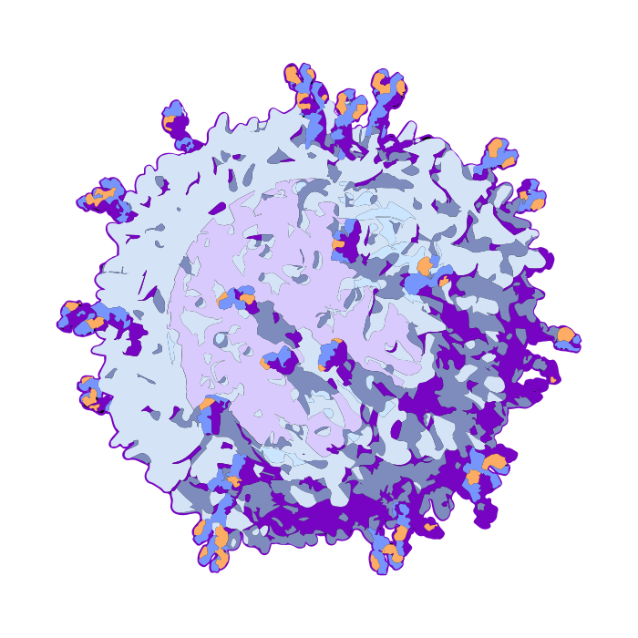
Antibodies are natural occurring proteins that will identify foreign actors within the body, such as viruses. In immunology, the target that antibodies recognize is called an antigen. An antigen can be the whole foreign element, or just a part of it, such as the spike protein in COVID-19. The antibody will bind to the antigen, forming an antibody-antigen complex.

A new promising technique in the drug design pipeline is in silico generative antibody design. Whereby, we use generative (AI) techniques to create suitable antibodies for a particular target.

Diffusion models are a class of generative models that have gained popularity for their ability to generate high-quality samples from complex distributions. They work by modeling the process of diffusion, where data points are gradually transformed into noise and then reconstructed back into data.

The most well know form of diffusion is image diffusion. Here during training the model will learn to denoise an image that has been corrupted with gaussian noise.

Recently it has been discovered that just like for creating new images from noise, diffusion models can be employed to create novel antibodies. Just like in the case of image diffusion they will during their training learn to reconstruct a corrupted random representation of an antibody. Then during inference novel antibodies can be generated from this noisy state.

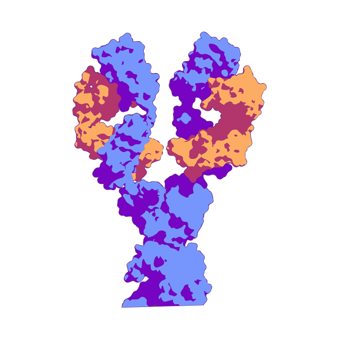
Antibody Structure

An antibody has a heavy and light polypeptide chain. Each chain has three complementary determining regions. Called CDR1, CDR2, CDR3. When referring to region 3 of the heavy chain we refer to CDRH3. The regions are highly variable loops and determine the binding specificity of the antibody. The rest of the antibody is more conserved. The CDRH3 region is the most variable. When talking about the backbone it refers to the N, C and CA atoms of each residue. The side chains are the rest of the atoms in the amino acid, and determine the amino acid type and it's properties.¹

Diffusion models

Diffusion models²³⁴ are characterized by a forward and backward process. The forward process will gradually add noise until the data is a multi variate Gaussian distribution. The backward process will learn to approximate the ground truth denoiser that will reconstruct the data from noise. Crucially in this work is the denoising step of the backward process. This is done by predicting the noise $\epsilon$ that was added to the data. The learned denoiser looks like:

where $\Sigma_\theta(x_t, t)$ is the variance predicted by the model at step $t$. For the covariance a time dependent profile is used so that this does not need to be learned.

$\mu_\theta(x_t, t)$ can be learned directly or we can learn the amount of noise that was added to $x_t$. This is done trough $\epsilon_\theta(x_t, t)$

Given the noisier sample $x_t$ and the predicted noise $\epsilon_\theta(x_t, t)$ the next step can be computed:

with $\alpha_t = 1 - \beta_t$ A higher $\alpha_t$ means more signal is preserved (less noise added). This is because it has an inverse relationship to $\beta$ which is the variance of the noise added at that time step. When the variance is low you retain more of the previous step in the forward process (when set to zero for example you copy over the step), when it is high you add more noise. $z$ is a point sampled from the prior distribution (typically a gaussian) $\sigma$ controls the amount of noise to add to the backward process, this is needed because each diffusion step is a stochastic process. In each forward diffusion step you sample from a conditional gaussian distribution, not only at $T$! If $\sigma_t$ would be zero then each step would be deterministic and we would lose sample diversity.

In this work the epsilon formulation will be used. The function to predict the added noise will be called EpsilonNet throughout this work. It will play a crucial role in applying the SIMS technique.

Foundations

Diffab

Diffab is a diffusion model that can generate new CDR-regions on an antibody-antigen complex. The model is trained on the SabDab dataset. During training one of the CDR-regions is masked out and the model has to reconstruct it. Diffab is from the paper "Antigen-Specific Antibody Design and Optimization with Diffusion-Based Generative Models" by Luo et. al ⁵.

Classically when diffusion is done for antibody design, the diffusion happens on the backbone representation of the antibody. After the backbone is generated an inverse folding model (such as proteinMPNN ⁶) is used to get the full amino acid sequence. Finally the side chains are added using a tool such as PyRosetta ⁷.

Diffab is different in that it does joint optimization of the structure and the sequence. The model will predict for each residue the $(x,y,z)$ position, rotation and the amino acid type. The model is equivariant to rotations and translations of the input structure.

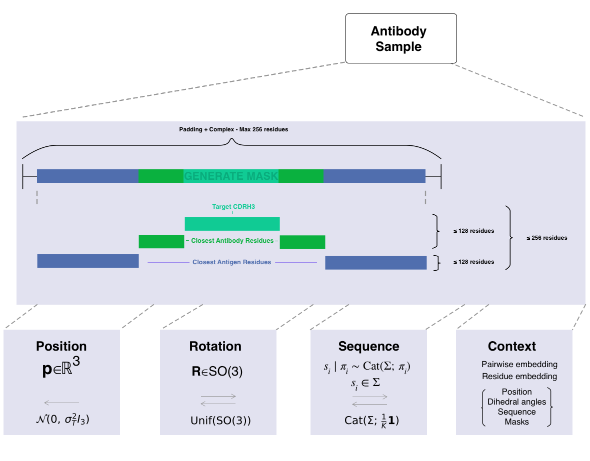
The following representation is used during diffusion:

• Position: $p \in \mathbb{R}^3$ Prior after $T$ steps: $\mathcal{N}(0,\,\sigma_T^2 I_3)$.

• Rotation: $R \in \mathrm{SO}(3)$ Prior after $T$ steps: $\operatorname{Unif}(\mathrm{SO}(3))$.

• Sequence: $s_i \mid \pi_i \sim \operatorname{Cat}(\Sigma;\,\pi_i),\quad s_i \in \Sigma$ Prior after $T$ steps: $\operatorname{Cat}(\Sigma;\,\tfrac{1}{K}\mathbf{1})$.

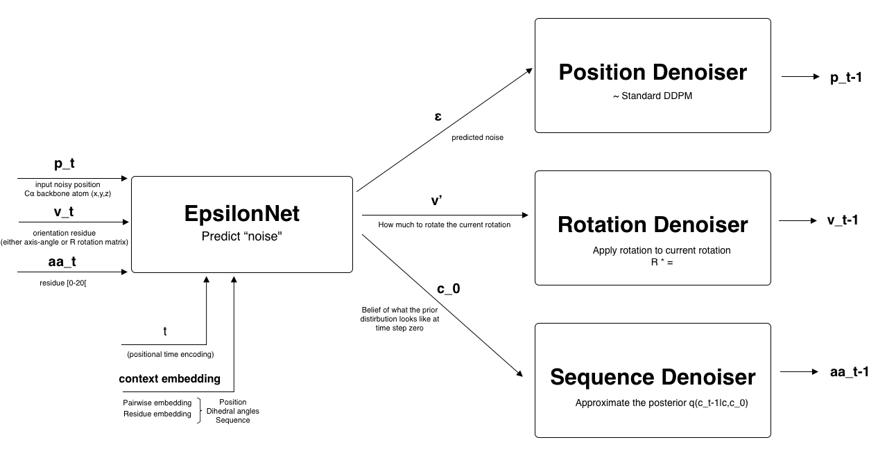
This structure is represented in Figure 1.

Figure 1Antibody-Antigen representationAntibody-Antigen representation for diffusion in Diffab.

Diffusion happens in the following way:

1. For step $t$: The position, rotation, sequence, context and time step are passed to the EpsilonNet. The "noise" is predicted for each of the three parts.
2. Each component is denoised using it's own denoiser. Adapted to the data representation. step $t-1$ is obtained.
3. This repeats for $T$ steps until a clean sample is obtained.

The epsilon of diffab has three different heads (the last part of the neural network):

• Position head: This head is responsible for predicting the noise added to each position. It thus predicts $\epsilon$ like standard diffusion.
• Orientation head: This head predicts the next orientation that has to be applied.
• Amino acid head: This head predicts a categorical distribution over the amino acid types for each residue. The distribution represents the prior belief of the original distribution. It is a categorical distribution.

Figure 2 available in the appendix illustrates the denoising process for one diffusion step.

SIMS

In the paper "Self-improving diffusion models with synthetic data" by Alemohammad et al. ⁸ the authors propose a new training paradigm for diffusion models that leverages self-synthesized data to improve the model's performance. The key idea is to use the model's own generated samples as a form of negative guidance during training, steering the model away from non-ideal synthetic data and towards the real data distribution.

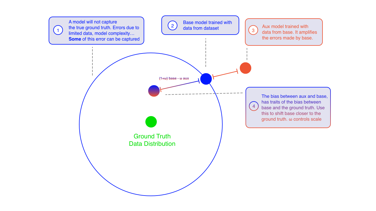
The method involves training two models: a base model and an auxiliary model. The base model is trained on the original dataset, while the auxiliary model is trained on synthetic data generated by the base model. During inference, the predictions from both models are combined to guide the sampling process. The combined prediction is given by:

The idea is that the bias between the base and auxiliary model has traits of the bias between the base and the ground truth. By subtracting the auxiliary model's prediction, the base model is nudged closer to the real data distribution. The parameter $\omega$ controls the strength of this guidance. Figure 3 and 4 illustrates the SIMS idea, they can be found in the appendix.

Methodology

Training the auxiliary model

A naive way to train an auxiliary model is to generate with the base model a new sample and pass it to the auxiliary model to train. You could either generate a new sample each time or form a dataset at the same time and reuse. The first approach makes training slow. The second although faster isn't ideal either since two models need to be loaded and there is still overhead.

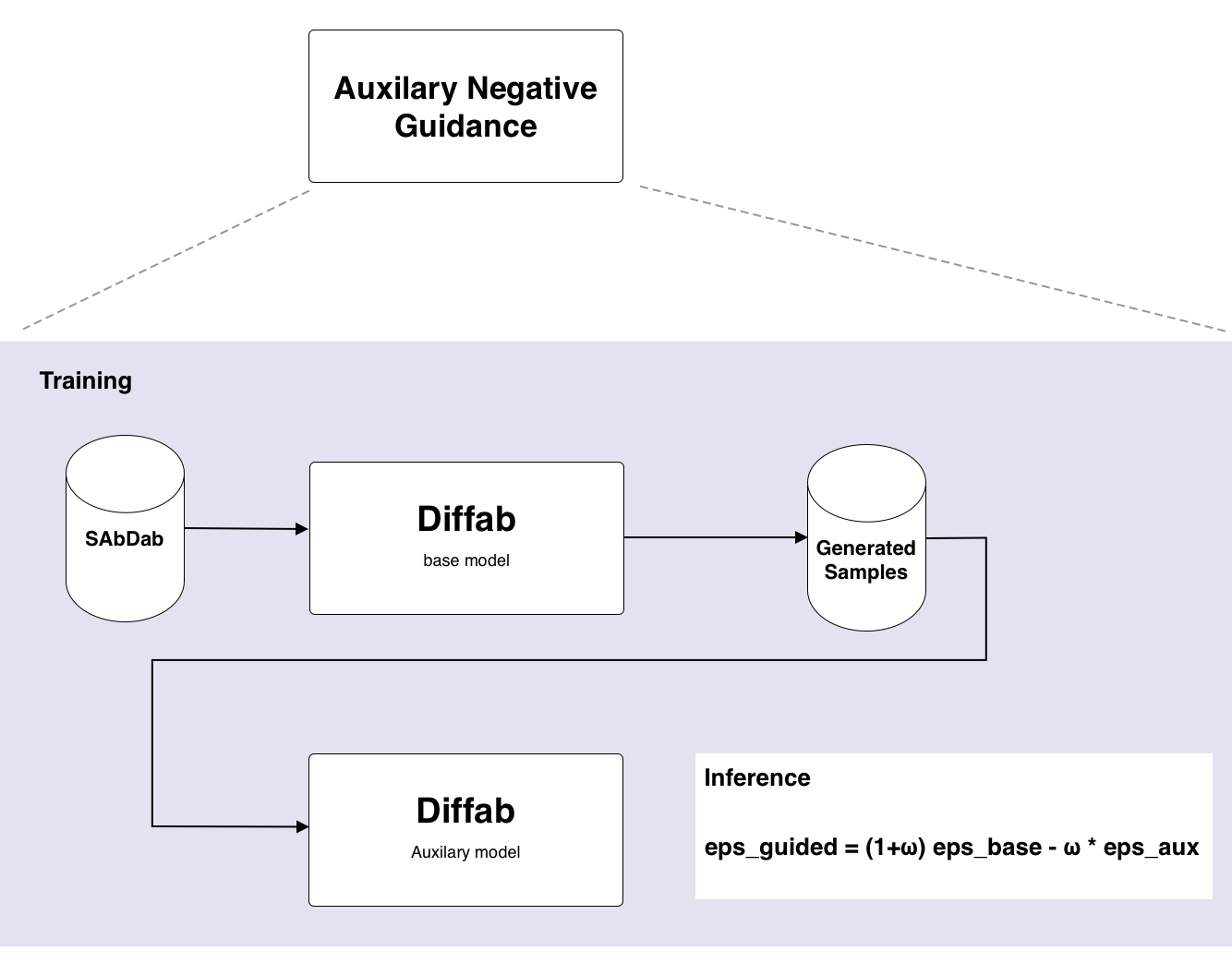
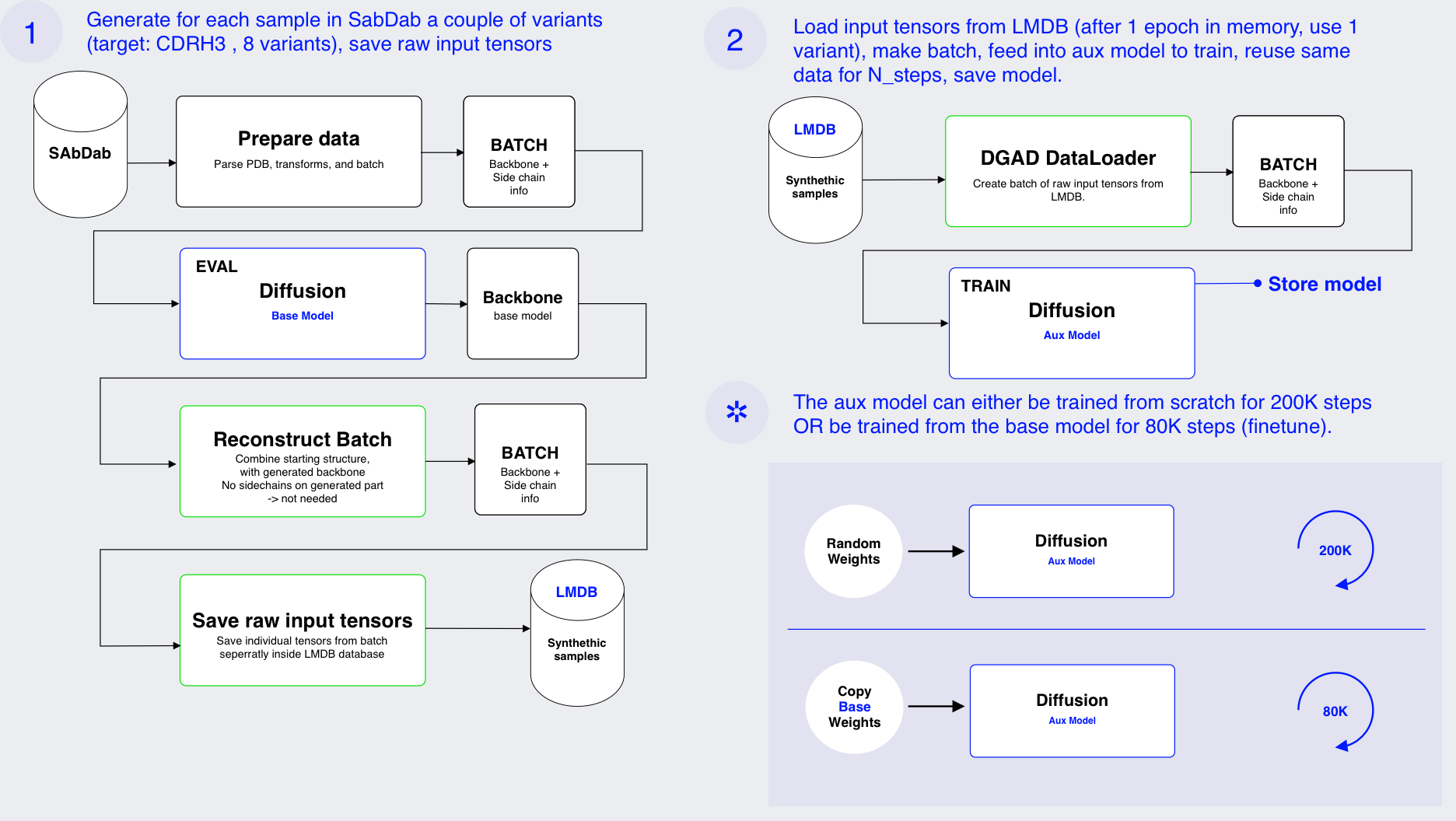
Therefore, to train the auxiliary model a two step approach was used:

1. First the base model is used to generate synthetic samples. These are saved in a data base. In stead of saving the processed PDB files, the direct tensor representation used by the model is saved. This eliminates the need to reprocess the data each time. It also avoids processing artifacts. This saves processing time when training the auxiliary model and also makes sure that data is not organized differently by processing artifacts. The data is saved in LMDB ⁹. LMDB is a key-value database that uses memory mapping to store data on disk. This makes it very fast to read data during training.
   • Note internally the model operates on backbone representation (position, rotation and sequence). When a sampling step is done during training diffab expects the full structure (including sidechains, masks, etc) as input. However after sampling the model only returns the backbone, afterwich it is reformatted to the full structure. Therefore an adapted sampling procedure was created that outputs the correct tensor representation for input into the model. This way the output of one model (the baseline) can be used directly as input for the auxiliary model.
2. Next the auxiliary model is trained on the synthetic data. A special dataloader is used that will read the data from the LMDB database and reconstruct the tensor representation used by the model.

This approach is outlined in Figure 5, which is available in the appendix.

Guidance on position

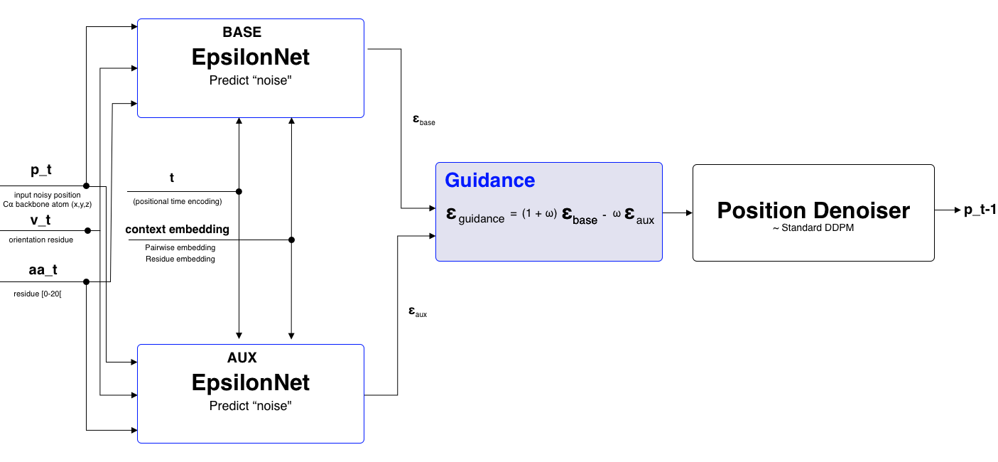
To evaluate the effectiveness of SIMS, the technique was applied on the position of each residue. This was chosen since the diffusion process on the position is similar too the diffusion process on images. The position is represented as a $(x,y,z)$ coordinate in 3D space. Applying guidance on the predicted noise for the position is a euclidian operation.

Within the diffab implementation the EpsilonNet predicts both position, rotation and amino acid type. During inference two epsilon nets are used, one for the base model and one for the auxiliary model. The guidance is only applied on the position part of the prediction. One drawback is that two models need to be loaded into memory. Before the position is denoised guidance is done on the predicted noise as shown in Figure 6.

Figure 6Guidance on positionGuidance on position during inference. Two epsilon nets are used, one for the base model and one for the auxiliary model. Guidance is applied on the predicted noise for the position only.

Extensions

Aside from simply applying guidance on the position, other types of guidance can be applied. The following extensions were considered:

Guidance on sequence The sequence is represented as a categorical distribution over the 20 amino acids. The EpsilonNet predicts for each residue a categorical distribution over the amino acids. This represents the prior belief of the original distribution. To apply guidance on this distribution we can use the following approach:

The last layer of the sequence head is a softmax layer. This means that the output is a probability distribution over the amino acids. To apply guidance this layer is removed next the logits are obtained. These logits are mixed using the SIMS formula. Next a softmax is applied again to obtain a valid probability distribution. Finally the denoising step is applied using this new distribution.

Guidance on rotation Applying guidance on rotation is not as straightforward as on position. The rotation is represented as a rotation matrix in SO(3). This means that the rotation is not a euclidian space. Therefore the guidance can not be applied directly on the prediction from the epsilon which predicts the next rotation that has to be applied. This way of applying has not been solved yet, however a possible solution could be:

• Conceptually we want to interpolate between two rotations. This can be done using lie algebra in tangent space. In this space we can apply guidance as a euclidean operation. Important to note is that the current rotation is applied on the sequence of rotations before it, therefore the predicted rotations need to be anchored at the current rotation.

Combined guidance Multiple types of guidance can be combined to improve the overall performance. In the hope that combining guidance on position, rotation and sequence will yield better results than just one type of guidance. To have reliable combined guidance it is important that each type of guidance has its own tuned guidance strength $\omega$. This is because the different types of data have different characteristics and scales. For example the position is a continuous variable in 3D space, while the sequence is a categorical variable. Therefore the impact of guidance on each type of data will be different.

Guidance schedule A guidance schedule can be used. This means that the guidance strength $\omega$ can be changed during the diffusion process for each type of guidance. For example: at the start no guidance can be applied to let the model 'warm up'. Next positional guidance can be increased in a linear way and kept steady for a few steps. Next rotational guidance can be turned on, and finally sequence guidance can be applied. The rationale is that the in this way the different types wont interfere. At the end you can also turn off guidance to let the model 'polish' the sample.

Metrics

Three metrics are used to evaluate the performance of the model: Root Mean Square Deviation (RMSD), which captures the difference between the generated and ground truth structure. Amino Acid Recovery (AAR), which measures the percentage of correctly predicted amino acids in the CDRH3 region. Finally, Perplexity Pseudo Log Likelihood (PPPL) is used to evaluate the biological plausibility of the generated sequences.

Results

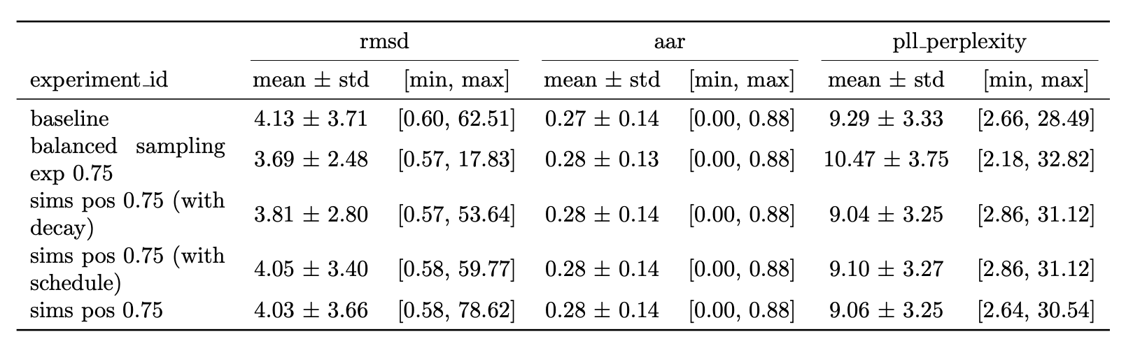
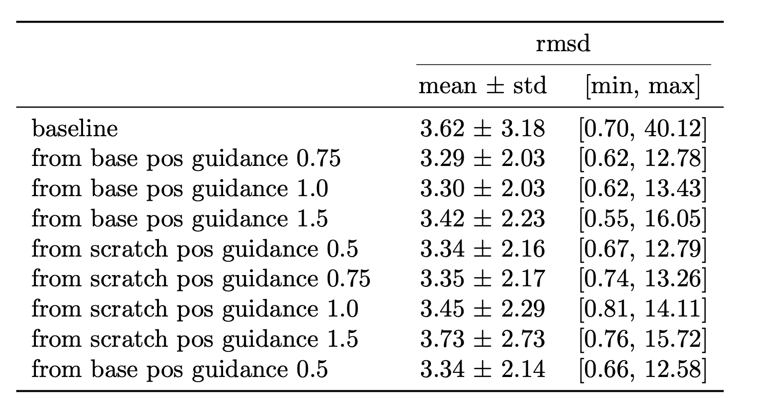
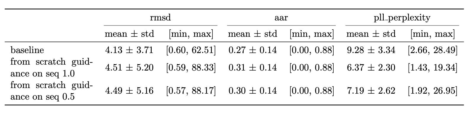
Figure 7 highlights the results of applying SIMS to Diffab. The results are obtained on a held out test set of 246 antibody-antigen complexes from SabDab. The RMSD is calculated on the generated CDRH3 region. For completeness an ablation study on the guidance strength $\omega$ is shown in Figure 8, provided in the appendix. Additionally study on sequence is shown in Figure 9. They are provided as supplementary material in the appendix, for more details see accompanying thesis.

Baseline is the base model trained from scratch using the newly discussed split and only on the CDRH3 region. Balanced sampling exp 0.75 is the same model but trained with a more balanced sampling strategy (using the word2vec style sampling). SIMS pos 0.75 is the base model with SIMS applied to position only, with a guidance strength of 0.75. SIMS pos 0.75 (with decay) is the same but using a decay. The decay is a linear decay starting from the initial guidance strength towards zero. The schedule is: no guidance for 10 steps then gradually increase guidance for position over 5 steps keep on for 40 steps. Then keep off.

The best results are obtained when using a guidance strength of 0.75 and without using decay or a schedule. The $0.75$ is obtained via an ablation study which can be found in the accompanying thesis along with more results on guidance on sequence and using different setups. This results in a $\sim8\%$ improvement over the baseline.

Most signal in the results can be obtained by looking at the RMSD since here guidance is only applied on the position which affects the structure. RMSD is better for all our implemented methods (lower is better).

Some small deviations in AAR are visible too this is because a joint epsilon net is used with three different heads so the a change in structure also affects the output of the sequence head of the epsilon net. The AAR for our methods (compared to baseline) is slightly higher (higher is better). Consequently the PPPL is also affected. For the guidance methods it's slightly lower (better).

Figure 7Results of applying SIMS to DiffabResults of applying SIMS to Diffab on a held out test set of 350 antibody-antigen complexes from SabDab. The RMSD is calculated on the generated CDRH3 region. The best results are obtained when using a guidance strength of 0.75 and without using decay or a schedule. This results in a ~8% improvement over the baseline. For each complex 8 samples were generated, the mean is computed over all samples, the std is the standard deviation and [min, max] is the range of values over all samples within the test set. Lower is better for rmsd and pll_perplexity, higher is better for aar.

Conclusion and future work

Future work

• Guidance mask in stead of equal guidance
  • In stead of applying equal guidance on each residue, a mask could be used to apply more guidance on residues that are further away from the ground truth. This mask could be learned.
• Classifier free guidance ¹⁰ using a learned guidance mask
  • Ommit using an auxiliary model. Instead train the base model with conditional information and with a mask that indicates which residues to apply more guidance on.
  • This can also be extended to learning the guidance mask trough reinforcement learning processes.

Conclusion

In this work the SIMS technique was applied to Diffab. The auxiliary model was trained using a two step approach to save training time. Guidance was applied on the position of each residue during inference. This resulted in a $\sim8\%$ improvement in RMSD on the CDRH3 region on a held out test set of 350 antibody-antigen complexes from SabDab. Successfully demonstrating the potential of guidance techniques to improve generative antibody design.

Appendices

Diffab

Figure 2Denoising processThe denoising process for one diffusion step in Diffab. The position, rotation, sequence, context and time step are passed to the EpsilonNet. The 'noise' is predicted for each of the three parts. Each component is denoised using it's own denoiser. This repeats for T steps until a clean sample is obtained.

SIMS

Figure 3SIMS IdeaSIMS idea: follow the numbers on the figure for an intuitive explanation.

Figure 4SIMS BasicSIMS: The sims procedure, training the auxiliary model and inference with guidance.

Training of the auxiliary model

Figure 5Auxiliary model trainingTraining the auxiliary model using a two step approach.

Ablation studies

Figure 8Ablation study on guidance strengthResults of ablation study on guidance strength omega. The results are obtained on a held out test set of 37 antibody-antigen complexes from SabDab. The RMSD is calculated on the generated CDRH3 region. The best results overall (taking in to account min/max) are obtained when using a guidance strength of 0.75. For each complex 8 samples were generated, the mean is computed over all samples, the std is the standard deviation and [min, max] is the range of values over all samples within the test set. Lower is better for rmsd.

Figure 9Ablation study on sequence guidanceResults of ablation study on guidance on sequence. The results are obtained on a held out test set of 351 antibody-antigen complexes from SabDab. The RMSD is calculated on the generated CDRH3 region. The best results overall (taking in to account min/max) are obtained when using a guidance strength of 1.0 on sequence only. For each complex 8 samples were generated, the mean is computed over all samples, the std is the standard deviation and [min, max] is the range of values over all samples within the test set. Lower is better for rmsd and pll_perplexity, higher is better for aar.

References